URFcomputation

Tutorials

Compute URFs

In the previous step we computed 32 streamlines for each domestic well and 100 steamlines for each irrigation well.

The following line will load the streamline data. However if you continue from the previous tutorial you can skip this.

load NPSAT_Streamline_Data

To compute the Unit Response Functions (URFs) for each streamline we need first to define an option structure, where dx is the discretization along the streamline, dt is the time discretization and Ttime is the total simulation time.

Here we will use 20 meters spatial discretization along the streamlines and 1 year temporal discretization and the total simulation time will be 200 years.

topt.dx = 20; % [m]
topt.dt = 1; % [years]
topt.Ttime = 200; % [years]

We allocate space to hold the URFs:

URFdm = zeros(size(XYZdm,1), topt.Ttime);

and compute the URFs for the domestic wells:

for i = 1:size(XYZdm,1)
    URFdm(i,:)=ComputeURF(XYZdm{i,1},Vdm{i,1},topt);
end

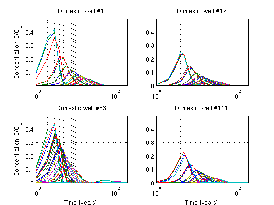
Below we randomly choose to plot the URFs for 4 dometic wells

figure(1);
id = well_id_dm == 1;
subplot(2,2,1);semilogx(URFdm(id,:)'); axis([0 200 0 0.5]); grid on
title(['Domestic well #' num2str(1)]);ylabel('Concentration C/C_{o}')
id = well_id_dm == 12;
subplot(2,2,2);semilogx(URFdm(id,:)'); axis([0 200 0 0.5]); grid on
title(['Domestic well #' num2str(12)])
id = well_id_dm == 53;
subplot(2,2,3);semilogx(URFdm(id,:)'); axis([0 200 0 0.5]); grid on
title(['Domestic well #' num2str(53)]);ylabel('Concentration C/C_{o}')
xlabel('Time [years]')
id = well_id_dm == 111;
subplot(2,2,4);semilogx(URFdm(id,:)'); axis([0 200 0 0.5]); grid on
title(['Domestic well #' num2str(111)]);xlabel('Time [years]')
drawnow

We repeate the steps above for the irrigation wells

URFir = zeros(size(XYZir,1), topt.Ttime);
for i = 1:size(XYZir,1)
    URFir(i,:)=ComputeURF(XYZir{i,1},Vir{i,1},topt);
end

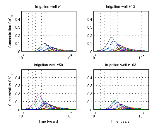
and plot randomly the URFs for 4 irrigation wells:

figure(2);
id = well_id_ir == 1;
subplot(2,2,1);semilogx(URFir(id,:)'); axis([0 200 0 0.5]); grid on
title(['Irrigation well #' num2str(1)]);ylabel('Concentration C/C_{o}')
id = well_id_ir == 13;
subplot(2,2,2);semilogx(URFir(id,:)'); axis([0 200 0 0.5]); grid on
title(['Irrigation well #' num2str(13)])
id = well_id_ir == 50;
subplot(2,2,3);semilogx(URFir(id,:)'); axis([0 200 0 0.5]); grid on
title(['Irrigation well #' num2str(50)]);ylabel('Concentration C/C_{o}')
xlabel('Time [years]')
id = find(well_id_ir == 103);
subplot(2,2,4);semilogx(URFir(id,:)'); axis([0 200 0 0.5]); grid on
title(['Irrigation well #' num2str(103)]);xlabel('Time [years]')
drawnow

Note how different the wells respond to tha same Unit ipnut loading function despite that the aquifer is homogeneous and the the recharges is somewhat uniform.