Tutorial: Complete NPSAT example

Problem Definition

This tutorial contains all the steps involved in the NPSAT construction and implementation phase.

Let assume that there is a hypothetical agricultural groundwater basin and there is a continuous contamination from the top due to the agricultural activities. The goal of this example is to obtain water quality Breakthought curves for the pumping wells. The aquifer receives primarily diffuse recharge from the various agricultural activities and partly from a stream. In the following we provide more details on that particular example.

Let's assume that the groundwater basin is a rectangular domain with dimensions 40 km x 10 km x 500 m. Let's also assume that there is a stream running the aquifer from the top to the bottom. The stream recharges the aquifer with variable rate that varies linearly between Nstrm = 1e-3 (y = 0) and Nstrm = 1e-2 (y = 40 km), while the average width of the stream is 60 m

We also assume that the groundwater recharge of the aquifer is devided into 4 zones:

First we will construct all the nessecery geometric features to describe the aquifer. For define the boundary of the domain as follows:

dom.Geometry = 'Polygon';
dom.X = [0 0 10000 10000 0 nan];
dom.Y = [0 40000 40000 0 0 nan];

Next we define the geometry of the stream

strm.Geometry = 'Line';
strm.X = [4970 4970 5030 5030 4970 nan];
strm.Y = [0 40000 40000 0 0 nan];
strm.DistMin = 50;
strm.DistMax = 500;
strm.LcMin = 50;
strm.LcMax = 500;

The aditional fields DistMin, DistMax, LcMin,LcMax are used to create a mesh with element sizes that vary linearly from 50 m at the stream to 500 m at a distance 500 m away from the stream. A nice graphical description of these fields can be found in the Gmsh tutorial t10.geo.

Last we will generate hypothetical locations for the wells.

The total amount of groundwater recharge in the hypothetical aquifer is 112600 m^3/day:

Therefore using a while loop we will generate as many wells as needed to make the pumping equal with the supply. (NPSAT is based on the steady state assumption, therefore the water balance have to be very close to zero)

This is a variable to strore the cumulative pumping

Q_tot = 0;

This is used to count the wells

cnt = 1;

This is used to store the x-y locations of the well in a matrix which will be used to compute the distanse between the new wells and the ones already generated. We do that because we do want two wells at a distance closer to 400 m.

wellsXY=[];

We split the wells into two categories: Domestic and Irrigation. Domestic wells have small pumping rates and short screens, while irrigation have large pumping rates and long screens During particle tracking we would need to know which wells are domestic and which are irrigation so we flag the irrigation wells with 1

well_flag =[];

clear well
while Q_tot < 112600
    wells(cnt,1).Geometry = 'Point';
    if cnt == 1
        xw = 400 + (9600 - 400)*rand; % we dont want the wells very close
        yw = 400 + (39600 - 400)*rand; % to the boundaries
    else
        while 1
            xw = 400 + (9600 - 400)*rand;
            yw = 400 + (39600 - 400)*rand;
            dst = sqrt((xw - wellsXY(:,1)).^2 + (yw - wellsXY(:,2)).^2);
            if abs(xw - 5000) < 400; continue;end
            if min(dst) > 400
                break
            end
        end
    end
    wells(cnt,1).X= xw;
    wells(cnt,1).Y= yw;
    wellsXY = [wellsXY;xw yw];
    if rand > 0.5;
        wells(cnt,1).Q = normrnd(1000,100);
        wells(cnt,1).desc = 'irr';
        wells(cnt,1).DistMin = 10;
        wells(cnt,1).DistMax = 500;
        wells(cnt,1).LcMin = 10;
        wells(cnt,1).LcMax = 200;
        wells(cnt,1).zt = 30;
        wells(cnt,1).zb = -150;
        well_flag(cnt,1) = 1;
    else
        wells(cnt,1).Q = normrnd(5,100);
        wells(cnt,1).desc = 'dom';
        wells(cnt,1).DistMin = 100;
        wells(cnt,1).DistMax = 500;
        wells(cnt,1).LcMin = 100;
        wells(cnt,1).LcMax = 500;
        wells(cnt,1).zt = 30;
        wells(cnt,1).zb = 0;
        well_flag(cnt,1) = 0;
    end

    Q_tot = Q_tot + wells(cnt,1).Q;
    cnt =cnt +1;
end

Next we will create a constructive solid geometry object that will hold the geometry of the aquifer

NPSAT = CSGobj_v2(2,1,10,300,10);%Dim,Npoly,Nline,Npoints,usertol

Read always first the domain outline

NPSAT = NPSAT.readshapefile(dom);

Read the stream

NPSAT = NPSAT.readshapefile(strm);

Read the wells

NPSAT = NPSAT.readshapefile(wells);

Next we will create the mesh

meshopt=msim_mesh_options;
meshopt.lc_gen = 1000;
meshopt.embed_lines = 1;
meshopt.embed_points = 1;
NPSAT.writegeo('npsat_example',meshopt);
gmsh_path = '/home/giorgos/gmsh-2.5.0-Linux/bin/gmsh';%'/usr/bin/gmsh';
NPSAT.runGmsh('npsat_example',gmsh_path,[])
[p2D MSH2D]=read_2D_Gmsh('npsat_example');

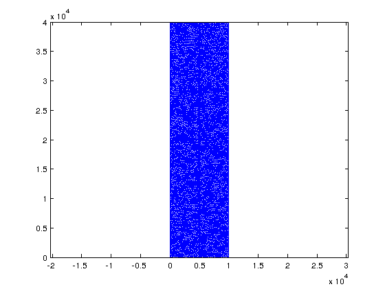
In Matlab it's easy to visualize small triangular meshes

triplot(MSH2D(3,1).elem(1,1).id, p2D(:,1), p2D(:,2));
axis equal

                    
                        
                    
                

Next we will extrude the 2D mesh to a 3D mesh of prism elements. We will use an initial uniform elevation of 30 m. This will be adapted to the actuall elevation during the flow simulation

top_elev = 30*ones(size(p2D,1),1);
bot_elev = -270*ones(size(p2D,1),1);
Nlay = 10;
t=linspace(0,1,Nlay);
[p3D MSH3D]=extrude_mesh(p2D, MSH2D, top_elev, bot_elev, t, 'linear');

Error   : Unknown string option 'General.RecentFile0'
Info    : Running '/home/giorgos/gmsh-2.5.0-Linux/bin/gmsh npsat_example.geo -2' [1 node(s), max. 1 thread(s)]
Info    : Started on Fri Mar 29 22:26:25 2013
Info    : Reading 'npsat_example.geo'...
Info    : Done reading 'npsat_example.geo'
Info    : Meshing 1D...
Info    : Meshing curve 1 (Line)
Info    : Meshing curve 2 (Line)
Info    : Meshing curve 3 (Line)
Info    : Meshing curve 4 (Line)
Info    : Meshing curve 5 (Line)
Info    : Meshing curve 6 (Line)
Info    : Meshing curve 7 (Line)
Info    : Meshing curve 8 (Line)
Info    : Meshing curve 9 (Line)
Info    : Meshing curve 10 (Line)
Info    : Done meshing 1D (0.436027 s)
Info    : Meshing 2D...
Info    : Meshing surface 1 (Plane, MeshAdapt)
Info    : Done meshing 2D (12.8088 s)
Info    : 22820 vertices 46393 elements
Info    : Writing 'npsat_example.msh'...
Info    : Done writing 'npsat_example.msh'
Info    : Stopped on Fri Mar 29 22:26:38 2013
Reading points...
Reading Elements...

Flow Simulation

In this example the aquifer is considered unconfined and the top layer elevation that correspond to the water table has to be adapted. Therefore to solve this problem we will use a while loop where during each loop we will assemble the conductance matrix and solve the system until the change in the water table is small.

Outside of the loop we will assemble the stresses and the boundary conditions First we compute the barycenters of the elements. We will assign the recharge for each element based on the location of the element barycenter

cc_elx = (p2D(MSH2D(3,1).elem.id(:,1),1) + ...
          p2D(MSH2D(3,1).elem.id(:,2),1) + ...
          p2D(MSH2D(3,1).elem.id(:,3),1))/3;
cc_ely = (p2D(MSH2D(3,1).elem.id(:,1),2) + ...
          p2D(MSH2D(3,1).elem.id(:,2),2) + ...
          p2D(MSH2D(3,1).elem.id(:,3),2))/3;

The elements associated with the recharge are all the triangles of the top layer. These are equal to the number of elements of the 2D mesh

Rch_Val = zeros(length(MSH2D(3,1).elem.id),1);

find which elements are in each zone and they are not stream elements

id =  cc_ely <= 10000 & (cc_elx < 4970 | cc_elx > 5030);
Rch_Val(id,1) = 1e-4;
id =  cc_ely > 10000 & cc_ely <= 20000 & (cc_elx < 4970 | cc_elx > 5030);
Rch_Val(id,1) = 2e-4;
id =  cc_ely > 20000 & cc_ely <= 30000 & (cc_elx < 4970 | cc_elx > 5030);
Rch_Val(id,1) = 3e-4;
id =  cc_ely > 30000 & (cc_elx < 4970 | cc_elx > 5030);
Rch_Val(id,1) = 4e-4;

F_rch(1,1).id = (1:length(MSH2D(3,1).elem.id))';
F_rch(1,1).val = Rch_Val;
F_rch(1,1).dim = 2;
F_rch(1,1).el_type='triangle';
F_rch(1,1).el_order='linear';

After the MSH2D is extruded into 3D two types of 2D elements are generated: triangles and quadrilaterals. The following index tell us that the indices in the field .id correspond to the following array MSH3D(F_rch(1,1).dim+1).elem(F_rch(1,1).id_el,1).id

F_rch(1,1).id_el=2;
%

Similarly to the diffuse recharge we will prepare a structure for the stream recharge

id = find(cc_elx >= 4970 & cc_elx <= 5030);

interpolate the rates for each element. The rates is actually a function of the y coordinate of the barycenter

Strm_Val = interp1([0 40000],[0.001 0.01], cc_ely(id,1));
F_rch(2,1).id = id;
F_rch(2,1).val = Strm_Val;
F_rch(2,1).dim = 2;
F_rch(2,1).el_type='triangle';
F_rch(2,1).el_order='linear';
F_rch(2,1).id_el=2;

Now we are ready to assemble the diffuse recharge. Since there are no General Head Boundary conditions the length of the stress vector will be equal to size(p3D,1)

F_rch_assmbled = Assemble_RHS(size(p3D,1), p3D, MSH3D, F_rch);

For the wells we will assign the pumping rates directly to nodes

F_wls = zeros(size(p3D,1),1);
for i = 1 : size(wells,1)
    dst = sqrt((wells(i,1).X - p3D(:,1)).^2 + (wells(i,1).Y - p3D(:,2)).^2);
    id_w = find(dst < 1);
    switch wells(i,1).desc
        case 'dom'
            % for domestic wells, the pumping is applied to layer 1 and 2
            F_wls(id_w(1:2),1) = -wells(i,1).Q/2;
        case 'irr'
            % for irrigation wells, the pumping is applied to layer 1 to 6
            % (However in reality one should assign pumping according the
            % the well depth distribution)
            F_wls(id_w(1:6),1) = -wells(i,1).Q/6;
    end
end

Next we need to define hydraulic conductivity and assign the constant head nodes (Dirichlet boundary conditions) We will assume a uniform horizontal hydraulic conductivity equal to 50 m/day and 0.5 m/day vertical hydraulic conductivity.

K = [50*ones(size(p3D,1),1) 0.5*ones(size(p3D,1),1)];

Note that by giving two columns to K matrix we define that Kx=Ky~=Kz. By giving 3 columns we actually instruct that Kx~=Ky~=Kz and by giving one column we assume Kx=Ky=Kz.

For the boundary conditions we will assume a small gradient which is typical in similar settings to out hypothetical example, where the hydraulic head at the south is 40 m and 30 m at the north boundary.

id_south = find(p3D(:,2) < 1);
id_north = find(p3D(:,2) > 39999);
CH = [id_south 40*ones(length(id_south),1);...
      id_north 30*ones(length(id_north),1)];

Solve Unconfine

This variable will help with the mesh adaptation procedure

Z = nan(size(p2D,1),Nlay);

and this will count the iterations

iter = 1;

Last we need to define few simulation options which are somehow self explainatory

simopt.dim = 3;
simopt.el_order = 'linear';
simopt.el_type = 'prism';
while 1
    % The following command assembles the conductance matrix
    [Kglo H]= Assemble_LHS(p3D, MSH3D(4,1).elem(1,1).id, K , CH, [], simopt);
    % so the system we need to solve actually is
    % Kglo * H = F_rch_assmbled + F_wls
    % Here we will use the default matlab method:
    % however with the system matrices available one can use any other solvers
    Hnew=solve_system(Kglo, H, F_rch_assmbled + F_wls);
    err(iter,1) = mean(abs(Hnew(1:size(p2D,1)) - p3D(1:size(p2D,1),3)));
    if err < 0.1
        break
    end
    %adapt the mesh so that the top layer is equal with the head elevation
    Z(:,1) = Hnew(1:size(p2D,1));
    Z(:,Nlay) = p3D((Nlay-1)*size(p2D,1)+1:end,3);
    Z =bsxfun(@times,Z(:,1),1-t) + bsxfun(@times,Z(:,end),t);
    p3D(:,3) = reshape(Z,Nlay*size(p2D,1),1);
end

Assembling Conductance ... x out of 36
                    1
                    2
                     .
                     .
                     .
                    35
                    36
Assembling Conductance ... x out of 36
                    1
                    2

                     .
                     .
                     .
                    35
                    36

In this particular example two iterations were adequate for the nonlinear problem to converge. (However this is not always the case. In fact in very complex cases the threshold of 0.1 might be to strict!)

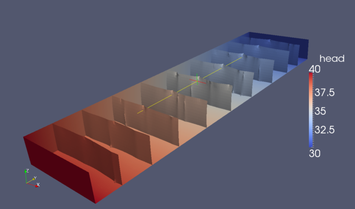
In Matlab we cannot visualize the solution so we will use paraview for that. First we have to write the solution in a format that paraview can read. Along with the mesh information we can assign properties on the nodes or cells. Here we will assign the hydraulic head solution, and the hydraulic properties, although the later are not very interesting for visualization.

The hydraulic heads are defined on the nodes:

propND(1,1).name = 'head';
propND(1,1).val = Hnew;
propND(1,1).type = 'scalars';

The hydraulic conductivity is uniform, therefore it doesnt really matter if it is defined on the nodes or the elements. However for illustration purposes we will define on the elements.

propND(2,1).name = 'HorCond';
propND(2,1).val = 50*ones(size(MSH3D(4,1).elem(1,1).id,1),1);
propND(2,1).type = 'scalars';
propND(3,1).name = 'VertCond';
propND(3,1).val = 0.5*ones(size(MSH3D(4,1).elem(1,1).id,1),1);
propND(3,1).type = 'scalars';
WriteVtkMesh('NPSAT_examp',MSH3D(4,1).elem(1,1).id,p3D,propND,[],'prism')

Writing Nodes coord...
Writing Elements...
Writing head...
Writing HorCond...
Writing VertCond...

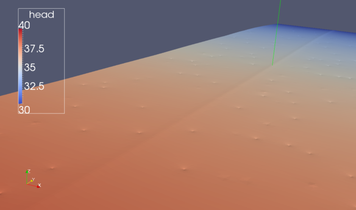
Paraview is a powerfull visualization tool. Here we show two plots. The first shows the iso surfaces of the head distribution and the second is a close look on the water table to see the effect of the adaptive mesh. Note the cone of depression for the wells as well as the shape of the water table along the stream.

Particle Tracking

Once the hydraulic head field is computed we can use it for particle tracking. In NPSAT we release particles from the sinks (wells) and using backward particle tracking we can identify their origin.

First we will generate the initial positions around the wells for the irrigation wells we will distribute the particles into 50 layers, with 4 particles each.

prtopt.radius = 10;% distance from the well point
prtopt.Nl = 25; %number of layers
prtopt.Nppl = 4; %number of particles per layer
[xp_ir yp_ir zp_ir well_id_ir] = distribute_particle_wells(wells(well_flag == 1), prtopt);

For the domasti wells we will distribute the particles into 8 layers, with 4 particles each.

prtopt.radius = 10;% distance from the well point
prtopt.Nl = 8; %number of layers
prtopt.Nppl = 4; %number of particles per layer
[xp_dm yp_dm zp_dm well_id_dm] = distribute_particle_wells(wells(well_flag == 0), prtopt);

Finally we need to adjust the data for the particle tracking algorithm. First we create a matrix which tell us how the elements are connected:

B = Build2Dmeshinfocpp(MSH2D(3,1).elem.id');

The current version of the particle tracking algorithm assumes that the 3D meshes are 2D meshes extruded into several layers. Therefore the x-y coordinates will be identical for all layers. In the particle tracking function we pass the node coordinates as follows:

XY = p2D(:,1:2);

Z = reshape(p3D(:,3),size(XY,1),Nlay);

each column of Z correspond to elevation of one layer.

Similarly for the hydraulic head and conductivity

Hnew = reshape(Hnew,size(XY,1),Nlay);
Kprt{1,1} = reshape(K(:,1),size(XY,1),Nlay);
Kprt{2,1} = reshape(K(:,2),size(XY,1),Nlay);

We also need to define few options. By pressing F1 while the cursor is on the function part_options you can see the explanation of the available options. Here we will use the default options, except the mode. We want to run the serial cpp because it is faster (see particle tracking tutorial).

trackopt = part_options;
trackopt.mode = 'cpp';

First we run backward particle tracking for the domestic wells:

[XYZdm Vdm exitflagdm]=ParticleTracking_main([xp_dm yp_dm zp_dm], XY, Z,...
                         MSH2D(3,1).elem.id, B, Hnew, Kprt, 0.1, trackopt);

and next we run the backward particle tracking for the irrigation wells:

[XYZir Vir exitflagir]=ParticleTracking_main([xp_ir yp_ir zp_ir], XY, Z,...
                        MSH2D(3,1).elem.id, B, Hnew, Kprt, 0.1,  trackopt);

Published with MATLAB® 7.14